CHAPTER 4 : DISCRETE PROBABILITY DISTRIBUTIONS
CHAPTER 4 : DISCRETE PROBABILITY DISTRIBUTIONSProbability distributions can be represented by tables or by formulas.The simplest type of probability distribution can be displayed in a table.Discrete Probability Distributions using PDF TablesEXAMPLE D1: Students who live in the dormitories at a certain four year college must buy a meal plan.They must select from four available meal plans: 10 meals, 14 meals, 18 meals, or 21 meals per week.The Food and Housing Office has determined that the 15% of students purchase 10 meal plan,45% purchase the 14 meal plan of students, 30% purchase the 18 meal plan ,10% purchase the 21 meal plan.a. What is the random variable? X Notation: P(Event) probability valueP(X 10 ) is the probability that a student purchases a meal plan with 10 meals per weekP(X 14 ) is the probability that a student purchases a meal plan with more than 14 meals per weekb. Make a table that shows the probability distributionThis table is called the PDFProbability Distribution Functionx Number of MealsProbability P(x)10We can create an extra column next tothe PDF table to help calculate the meanxP(x)141821c. Find the probability that a student purchases more than 14 meals:d. Find the probability that a student does not purchase 21 meals.e. On average, how many meals does a student purchase per week in their meal plan?Calculate the mean.Mean Expected Value: µ SxP(x) µ f. Write a sentence that interprets the mean in the context of the problem.NOTE that it is acceptable that the mean is not whole number; it can have a fraction or a decimal.Page 1
CHAPTER 4 : DISCRETE PROBABILITY DISTRIBUTIONSDiscrete Probability Distributions using PDF Tables PDF: Probability Distribution FunctionAll probabilities are between 0 and 1, inclusive AND All probabilities must sum to 1. Mean Expected Value µ SxP(x)Interpreted as a long term average over many observationsFormula is a “weighted” average where each value is “weighted” according to how likely is its to occur Standard Deviation s å (x -µ )2P( x)Measures variation in the probability distributionFormula is a “weighted” average of the squared distances between each data value and the mean Variance (standard deviation)2 s2 å (x -µ )2P( x )Measures variation in the probability distributionBefore widespread technology, variance was easier to calculate than standard deviationVariance is used in some types of “statistical tests” instead of standard deviationEXAMPLE D2: The Highway Commissioner wants to know how many people are in cars that use thecarpool lanes on Ocean Expressway. The best way to estimate occupancy of a car accurately is with humanobservers; electronic methods often are not accurate.A team of “observers” is sent to watch the highway from overpasses and count the number of occupants in asample of cars passing below the overpass. Based on the data, the number of occupants in cars in thecarpool lane on Ocean Expressway follows the probability distribution below.XP(X)10.120.530.340.1a. Draw a relative frequency histogramof this probability distributionb. Find the expected value andwrite a sentence that interprets its meaningin the context of the problemc. Find the variance s2 å (x -µ )20P(x) and the standard deviation: s 12å (x -µ )324 peopleP( x)by doing the calculation step by step using the table.NOTE: We’ll do this in class together once. After that we’ll always use our calculator to do this for us.d. Use your calculator 1VarStats to find the mean, standard deviation , and variance.Page 2
CHAPTER 4: DISCRETE PROBABILITY DISTRIBUTIONS USING PDF TABLESEXAMPLE D3: At the county fair, a booth has a coin flipping game.You pay 1 to flip three fair coins.If the result contains three heads, you win 4. If the result is two heads, you win 1. Otherwise there is no prize.We are interested in the net amount of money gained or lost in one game.a. Define the random variable and the values it can have.b. Write the PDF for the amount gained or lost in one game.c. Find the expected value for this game (Expected NET GAIN OR LOSS)d. Find the expected total net gain or loss if you play this game 50 times.EXAMPLE D4: Suppose you play a different game. In this game, you flip a biased coin twice.A biased or unfair coin has different probabilities for landing on heads and tails.Suppose that for this coin, P(HEAD) 2/3 and P(TAIL) 1/3.In this game you do not pay in order to play.You toss the coin twice, and then win or lose according to the following:win 3 if you toss two tailswin 1 if you toss two headspay (lose) 2 if you toss one head and one tail.We are interested in the net amount of money gained or lost in one game.a. Define the random variable and the values it can have.b. Write the PDF for the amount gained or lost in one game.c. Find the expected value for this game (Expected NET GAIN OR LOSS)Page 3
CHAPTER 4 : DISCRETE PROBABILITY DISTRIBUTIONS USING PDF TABLESEXAMPLE D5: In this game we roll ONE fair EIGHT SIDED DIE once.(The eight sides of the die arenumbered 1, 2, 3, 4, 5, 6, 7, 8 and the die has an equal chance of landing on each side.)Suppose that you win 6 if you roll an 8, win 2.50 if you roll a 2,lose 2 if you roll an odd number, andif you roll a 4 or 6 you neither win anything nor lose anything.We are interested in the monetary outcome for one game.a. Define the random variable and the values it can have.b. Write the PDF for the amount gained or lost in one game.c. Find the expected value for this game (Expected NET GAIN OR LOSS)d. Find the expected total net gain or loss if you play this game 100 times.EXAMPLE D6 A real estate developer is presenting plans to the Planning Commissioner for a development ofhouses and apartments he proposes to build. He needs to estimate the impact on the local schools so he mustestimate the number of children expected to attend the schools. He hires a statistician who studies thedemographics of the neighborhood and of similar housing developments; she provides the estimates below.Let X the number of school age children per household.a. Find the expected number of children per householdb. Find the expected number of school age children in the new housing development if 120 housing units are built.XP(X)00.3010.18230.1540.0850.056 ore more0Page 4
CHAPTER 4 :BINOMIAL PROBABILITY DISTRIBUTIONThe Binomial Distribution is a special discrete probability distribution that arises often in problems.A BINOMIAL probability experiment has a fixed number n of repeated trials each trial has outcomes that we can classify as “success or “failure” outcome of trials are independent (Outcome of a trial does not influence outcome of future trials)The probability of success on a single trial, p, is constant (the same) for all trialsWe are interested in the number of successes, x, in n trialsNotation: X B(n,p)EXAMPLE B1: A college claims that 70% of students receive financial aid. Suppose that 4 students at thecollege are randomly selected. We are interested in the number of students in the sample who receive financial aid.X p the probability that a student receives financial aid:X B(4, 0.7) : Binomial with n 4 and p 0.7X0P(x)p q 1 p Ways to get x successes in n trialsn 4x 1AbcdaBcdabCdabcD1234n 4x 2ABcdA bC dAbcDaBCdaB cDabCDn 4x 3aBCDAbCDABcDABCda. Find the probability that AT MOST 2 of the students in the sample receive financial aid:b. Find the probability that AT LEAST 3 of the students in the sample receive financial aid:c. Find the mean and the standard deviation using the shortcut formulas for the binomial distribution:µ np;s npqwhere q 1 - ponly for Binomial distribution.These shortcut formulas for µ and s give the same results as the definitions µ SxP(x) , s Formulas for Binomial Distribution:X B(n,p)å (x -µ ) P(x)2P(X x) nCx px (1 p) n xP(X x) is the probability of obtaining x successes in n independent trialµ np ;n Cxs npqwhere q 1 - ponly for binomial distribution.represents the number of ways (patterns) in which it is possible to get x successes in n trialsnC xænö ç ç x è øn!x!(n - x)!Where n! n(n 1)(n 2)(n 3). . .(3)(2)(1) for integers n 0Example 4! (4)(3)(2)(1) 24 3! (3)(2)(1) 6 2! (2)(1) 6also 0! 1 by definition(4)(3)(2)(1)4!4! 64C 2 nCx using calculator MATH PROB nCr :2!(4 - 2)! (2!)(2!) (2)(1)(2)(1)Example: 4 MATH PROB nCr 2 ENTERPage 5
CHAPTER 4: BINOMIAL PROBABILITY DISTRIBUTIONP(X x)binompdf (n,p,x)Binomial Distribution TI 83, 84 CalculatorUse binompdf or binomcdf found at2nd Distrbinompdf : P(X value) probability distribution functionbinomcdf : P(X value) cumulative distribution functionP(X x)binomcdf (n,p,x)P(X x)binomcdf (n,p,x 1)P(X x)1 binomcdf (n,p,x)P(X x)1 binomcdf (n,p,x 1)TI-89 APPS; B2:1: FlashApps; highlight Stats/List Editor ENTER F5: nes-for-surveys-in2016/?utm source Pew Research Center&utm campaign 4a62041804-Methods Newsletter for June6 24 surveys-in2016/?utm source Pew Research Center&utm campaign 4a62041804-Methods Newsletter for June6 24 2015Many of the major survey organizations that conduct “public opinion polls” gather their data through telephonesurveys. These types of polls include political polls, polls about current events, and other subjects aboutdemographics, lifestyle, economic issues, and more. In recent years, these survey organizations have had tochange their data gathering techniques, as sampling from landline phones only will no longer provide a samplethat is representative of the population.Kyley McGeeney, a research methodologist at Pew Research Center, wrote that “All major survey organizationsthat conduct telephone surveys include cellphones in their samples. They have to, because the kinds of peoplewho rely only on a cellphone are different from those reachable on a landline, even though being cellphone-onlyis becoming more mainstream. Cellphone-only individuals are considerably younger than people with a landline.They tend to have less education and lower incomes than people with a landline. They are also more likely to beHispanic and to live in urban areas. For this reason, excluding cellphones from a poll – or not including enough ofthem – would provide a sample that is not representative of all U.S. adults.”Drew DeSilver at Pew Research Center cites that 65.7% of 25- to 29-year-olds live in wireless-only householdsand do not have landlines.Suppose we took a sample consisting of 100 people age 25-29 and we are interested in counting the number ofpeople in the sample who have only cell phone service.X (description)p (description)p (value)X a. Find the probability that 60 have only cell phone serviceb. Find the probability that at most ( )60 have only cell phone servicec. Find the probability that less than 60 have only cell phone serviced. Find the probability that the number who have only cell phone service exceeds (is more than) 60e. Find the probability that at least (³) 60 have only cell phone servicef. Find the probabilitythat exactly half of the people in the sample have only cell phone servicePage 6
CHAPTER 4: BINOMIAL PROBABILITY DISTRIBUTIONP(X x)binompdf (n,p,x)Binomial Distribution TI 83, 84 CalculatorUse binompdf or binomcdf found at2nd Distrbinompdf : P(X value) probability distribution functionbinomcdf : P(X value) cumulative distribution functionP(X x)binomcdf (n,p,x)P(X x)binomcdf (n,p,x 1)P(X x)1 binomcdf (n,p,x)P(X x)1 binomcdf (n,p,x 1)TI-89 APPS; 1: FlashApps; highlight Stats/List Editor ENTER F5: DistrEXAMPLE B3: Make sure that the probability of success matches the definition of a successA recent study showed that about 60% of California voters voted by mail. Suppose we are selecting a randomsample of 75 voters and we are interested in the number of people in the sample who vote in person at the polls.X (description)p (description)p (value)X a. Find the probability that more than 25 of the voters in the sample voted in person at the polls.b. How many people in the sample would you expect to vote in person at the polls.EXAMPLE B4: PRACTICE Try-It 4.13 Introductory Statistics from Openstax download for free at www.openstax.orgAbout 32% of students participate in a community volunteer program outside of school.Suppose that 30 students are selected at random.X the number of students who participate in a community volunteer program outside of school X a. Find the probability that at most 14 participate in a community volunteer program outside of schoolb. Find the probability that at least 15 participate in a community volunteer program outside of schoolc. Find the probability that more than 20 participate in a community volunteer program outside of schoold. For many samples of 30 students, on average, what is the expected number per sample who participate in acommunity volunteer program outside of school?e. Find the standard deviationNOTE: Recognizing Scientific Notation on your Calculator:Sometimes probabilities are very small numbers.If the number is very close to 0, your calculator automatically uses scientific notation:0.000068 6.8 x 10⁻⁵ appears on the calculator as 6.80000000E-54.26710E-6 4.26713x 10⁻⁶ 0.00000426713 (move decimal point left 6 places)Page 7
They must select from four available meal plans: 10 meals, 14 meals, 18 meals, or 21 meals per week. The Food and Housing Office has determined that the 15% of students purchase 10 meal plan, 45% purchase the 14 meal plan of students, 30% purchase the 18 meal plan ,10% purchase the 21
Joint Probability P(A\B) or P(A;B) { Probability of Aand B. Marginal (Unconditional) Probability P( A) { Probability of . Conditional Probability P (Aj B) A;B) P ) { Probability of A, given that Boccurred. Conditional Probability is Probability P(AjB) is a probability function for any xed B. Any
Part One: Heir of Ash Chapter 1 Chapter 2 Chapter 3 Chapter 4 Chapter 5 Chapter 6 Chapter 7 Chapter 8 Chapter 9 Chapter 10 Chapter 11 Chapter 12 Chapter 13 Chapter 14 Chapter 15 Chapter 16 Chapter 17 Chapter 18 Chapter 19 Chapter 20 Chapter 21 Chapter 22 Chapter 23 Chapter 24 Chapter 25 Chapter 26 Chapter 27 Chapter 28 Chapter 29 Chapter 30 .
Chapter 5: Discrete Probability Distributions 158 This is a probability distribution since you have the x value and the probabilities that go with it, all of the probabilities are between zero and one, and the sum of all of the probabilities is one. You can give a probability distribution
Random variables (discrete and continuous) . concepts from information theory, linear algebra, optimization, etc.) will be introduced as and when they are required (IITK) Basics of Probability and Probability Distributions 2. Random Variables . Uniform: numbers de ned over a xed range Beta: numbers between 0 and 1, e.g., probability of head .
TO KILL A MOCKINGBIRD. Contents Dedication Epigraph Part One Chapter 1 Chapter 2 Chapter 3 Chapter 4 Chapter 5 Chapter 6 Chapter 7 Chapter 8 Chapter 9 Chapter 10 Chapter 11 Part Two Chapter 12 Chapter 13 Chapter 14 Chapter 15 Chapter 16 Chapter 17 Chapter 18. Chapter 19 Chapter 20 Chapter 21 Chapter 22 Chapter 23 Chapter 24 Chapter 25 Chapter 26
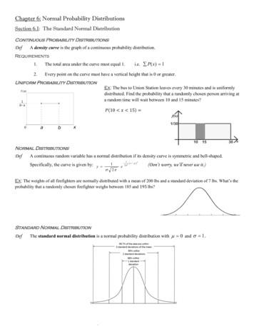
Chapter 6: Normal Probability Distributions Section 6.1: The Standard Normal Distribution Continuous Probability Distributions Def A density curve is the graph of a continuous probability distribution. Requirements 1. 1The total area under the curve must equal 1. i.e. Px 2. Every point
Network Security, WS 2008/09, Chapter 9IN2045 -Discrete Event Simulation, SS 2010 22 Topics Waiting Queues Random Variable Probability Space Discrete and Continuous RV Frequency Probability(Relative Häufigkeit) Distribution(discrete) Distribution Function(discrete) PDF,CDF Expectation/Mean, Mode, Standard Deviation, Variance, Coefficient of Variation
2.1 Sampling and discrete time systems 10 Discrete time systems are systems whose inputs and outputs are discrete time signals. Due to this interplay of continuous and discrete components, we can observe two discrete time systems in Figure 2, i.e., systems whose input and output are both discrete time signals.


