A Quick Guide To Using Excel 2007’s Regression Analysis Tool
A Quick Guide to Using Excel 2007’sRegression Analysis Tool
Table of ContentsPageThe Analysis Toolpak . 1If the Add-In is ALREADY Installed . 1If the Add-In is NOT ALREADY Installed . 1Run a Multiple Regression: An ExampleIntroduction. 2Steps to Follow. 21. Rearrange the Data as Necessary . 22. Open the Regression Analysis Tool . 33. Complete the “Regression” Dialog Box. 44. Run the Regression Analysis and View the Results . 5The Regression Results Areas. 6Run Another Regression Analysis . 69-11-2009
Using Excel 2007’s Regression Analysis ToolThe Analysis TookpakExcel 2007 has a built-in regression analysis tool that’s packaged as part of its “AnalysisToolpak”. The Analysis Toolpak is a standard component of Excel. Microsoft makes itavailable as an Excel add-in. If you loaded your copy of Excel on your computer, youmay recall that you had a choice during the installation process whether or not toinclude add-ins such as the Analysis Toolpak.If the Add-In is ALREADY InstalledIf the Analysis Tookpak add-in is already installed, you’ll see an “Analysis” group in the“Data” tab of Excel’s ribbon. Click the “Data Analysis” button in that group to open the“Data Analysis” dialog. Then scroll down to find the “Regression” option.The Analysis Toolpak add-in is installed in Excel 2007 on all FuquaNet MBA PCs.If the Add-In is NOT ALREADY InstalledIf you’re using your own computer and you do not yet have the add-in installed, followthese steps to install it:1. Close Excel if you have it open.2. Make your installation medium (probably a CD) available to your computer.3. Restart the Excel installation routine. (Note that you need not reinstall Excelentirely.)4. Find the option to modify the installation and choose the Analysis Tookpak as anadd-in that should be activated.5. Exit the installation process.6. Open Excel and confirm that the “Data Analysis” dialog is available (see above).1
Run a Multiple Regression: An ExampleIntroductionThis example walks you through how to use Excel 2007’s built-in regression tool toanalyze whether information collected by the Mrs. Smyth’s Gourmet Frozen Fruit PieCompany (price, advertising, competitors’ pricing, etc.) can predict company pie sales.The worksheet with pie data is partially shown in the illustration below. There are tencolumns of data with forty-eight records.For this example regression operation:We use as the predictor variables (the independent or X variables) the data forPrice, Ads, Comp Price, Income, Population, and Time Var.We use as the predicted variable (the dependent or Y variable) the data for UnitSales. Unit Sales holds actual sales data.Steps to Follow When Running a Regression with Excel1. Rearrange the Data as NecessaryWith Excel’s regression tool the independent X variables you use in your analysis mustbe located together in the worksheet. There must be no blank columns or columns withnon-relevant data interrupting the range of X variables. The dependent Y variable neednot be located adjacent to the X variables, but all Y variable values must be in a singlerange. These location specifications are required by Excel’s built-in regression tool.2
For the data in our sample, the data need not be rearranged. The X variables are togetherin Columns F through K and the Y variable values are all in Column E.Columns not used inthis regression.The dependent,Y variable.Independent, X variables,located together in theworksheet.2. Open the Regression Analysis ToolIn the “Data” tab on Excel’s ribbon find the “Analysis” group and click the “DataAnalysis” button.Excel opens its “Data Analysis” dialog. Scroll down and find the “Regression” option.Click OK.3
Excel 2007’s “Regression” dialogdisplays. This is the sole interfaceto Excel’s regression tool. Allyour interaction with Excel’sregression tool happens in thisdialog.3. Complete the “Regression” Dialog Box- Specify “Unit Sales” as the “Input Y Range”. Include the column header cell (the cellthat holds the text “Unit Sales”) in your range specification1.- Specify the range of data in Columns F through K as the “Input X Range”. Include onlyone row of column headers with your range specification (that is, include onlythe labels directly above the data).- In the “Regression” dialog box make sure the Labels box is checked. With this optionchecked Excel will recognize that the first cell in each column of data is a datalabel.1In this selection operation be careful to select data and header only and not an entire column. Here’s aneasy way to select just the contiguous data from a column of data: Click the top cell. Depress the SHIFTkey. Tap the End key and then tap the down arrow key. Excel selects all data down the column until itreaches the first empty cell in the column.4
- Direct Excel to put its results on a new worksheet by choosing the option NewWorksheet Ply.- For outputs, select Residuals, and Standardized Residuals.With data ranges and choices specified, your dialog should now look like the one below.4. Run the Regression Analysis and View the ResultsWith the dialog box options completed as described above, click OK to execute theregression.The New Worksheet Ply default output option means that Excel locates the regressionoutputs on a new, separate worksheet that it creates and puts to the left of the worksheetthat holds the original data.Excel completes the regression analysisleaving a large range of the worksheetselected. Click any cell to turn off therange selection. Because the Regressiontool generates many outputs on a singlesheet, you may want to use Excel’s ZoomControl option to reduce the newworksheet size in order to get a view ofhow the outputs are arranged.5
Widen the columns on the new worksheet in order to see all the text results properly. Aquick way to do this is to select the blank square at the intersection of the row numbersand column headers (to select the entire worksheet), and then double-click the dividingline between any two column headers. Excel widens each column so the widest entry inthat column displays completely.The Regression Results AreasSelecting the Residuals, and Standardized Residuals options in the “Regression” dialogproduces the output partially shown below.In this view columns have been widened to show the results completely.Excel labels the output areas “SUMMARY OUTPUT”, “ANOVA”, and “RESIDUALOUTPUT”.Run Another Regression AnalysisPerhaps after viewing the results of the first analysis you decide you’d like to runanother regression analysis using different variables or a different combination ofvariables. To do so, go through the same steps as above. Excel adds a new worksheet tohold the new results. The original results (from the first analysis) remain in place.End6
Sep 11, 2009 · Using Excel 2007’s Regression Analysis Tool The Analysis Tookpak Excel 2007 has a built-in regression analysis tool that’s packaged as part of its “Analysis Toolpak”. The Analysis Toolpak is a standard component of Excel. Microsoft makes it available as an Excel add-in. If you loaded your copy of Excel on your computer, youFile Size: 314KB
work/products (Beading, Candles, Carving, Food Products, Soap, Weaving, etc.) ⃝I understand that if my work contains Indigenous visual representation that it is a reflection of the Indigenous culture of my native region. ⃝To the best of my knowledge, my work/products fall within Craft Council standards and expectations with respect to
LOGIQ e GE Healthcare. 2 LOGIQ e Quick Card The Quick Card is a quick reference to operation. Please refer to Basic User Manual for detailed information. Control Panel 1 15 14 6 7 13 12 5 11 4 10 3 9 2 8. LOGIQ e Quick Card 3 The Quick Card is a quick reference to operation. Please refer to Basic User Manual for detailed information.
LOGIQ e Quick Card 10 11 LOGIQ e Quick Card The Quick Card is a quick reference and not does not replace the User Manual. Please refer to the Basic User Manual for complete safety and operation information. The Quick Card is a quick reference and not does not replace the User Manual. Please refer to the Basic User Manual for complete safety
akuntansi musyarakah (sak no 106) Ayat tentang Musyarakah (Q.S. 39; 29) لًََّز ãَ åِاَ óِ îَخظَْ ó Þَْ ë Þٍجُزَِ ß ا äًَّ àَط لًَّجُرَ íَ åَ îظُِ Ûاَش
Collectively make tawbah to Allāh S so that you may acquire falāḥ [of this world and the Hereafter]. (24:31) The one who repents also becomes the beloved of Allāh S, Âَْ Èِﺑاﻮَّﺘﻟاَّﺐُّ ßُِ çﻪَّٰﻠﻟانَّاِ Verily, Allāh S loves those who are most repenting. (2:22
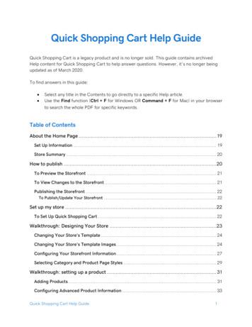
Quick Shopping Cart Help Guide 1 . Quick Shopping Cart Help Guide . Quick Shopping Cart is a legacy product and is no longer sold. This guide contains archived Help content for Quick Shopping Cart to help answer questions. However, it's no longer being updated as of March 2020. .
1.4 Fonts Font sizes Point size Latex cmd User-de ned * Sample 5 6 \tiny \xxxsmall the quick brown fox 7 8 \scriptsize \xxsmall the quick brown fox 8 10 \footnotesize \xsmall the quick brown fox 9 11 \small \small the quick brown fox 10 12 \normal \normal the quick brown fox
Quick-Build Warehouse SBH2600, height 2.6m 6 Quick-Build Warehouse SBH3000, height 3.0m 8 Quick-Build Warehouse SBH4000, height 4.0m 10 Quick-Build Warehouse SBH4800, height 4.8m 12 Useful accessories 14 Your individual Quick-Build Warehouse


