Excel 2007 Formulas And Functions - Mandelasshoima.ac.ug
Excel 2007Formulas and FunctionsFor additional help with this or other software programs, contact the Center forTeaching and Learning (ctl@mcmail.maricopa.edu)480-461-7690Mesa Community CollegeChristine Held1
This manual was created using excerpts from Introduction to Excel 2002, created by theTechnology Training Services department at the Maricopa Community College District Office.Other portions of this manual were created by Christine Held, BPC/CIS Faculty at MesaCommunity College.Some picture excerpts were supplied by Thomson-Course Technology 2007.Some text and pictures were inserted directly from the Microsoft Excel Help feature.Mesa Community CollegeChristine Held2
Learning Objectives:Adding Comments to CellsAbsolute vs. Relative Cell ReferencesCreating multiple worksheets and adding 3D referencesCreating Conditional formattingGrouping WorksheetsDate FunctionsUsing If FunctionsNaming RangesRound FunctionUsing Min, Max and Average functionsAuditing FormulasMesa Community CollegeChristine Held3
Review Exercise: Create the following worksheet1. Create the following worksheet and used the formulas as displayed below. Name thesheet “Quarter 1”.2. Save as Quarterly Budget.Formulas to be used:Mesa Community CollegeChristine Held4
ADDING COMMENTS TO CELLSExcel has a useful feature call COMMENTS. The comments are notes attached to a specific cellin a worksheet. They are useful as references or as a help to others who use the worksheet.When a note is attached to a cell, a small triangular marker displays at the top right corner ofthe cell. These markers, as well as the comments, do not automatically print.Using the Review Tab, this is what the comment menu choices are:AddCommentsto a CellAdd Comments to a Cell1. Select the cell to contain the comment.2. From the Review tab, select the insert Comment icon. A text box willdisplay. Tip: Right click and select Insert Comment.3. Type the text of the comment in the text box.4. Click anywhere outside the text box to close it.ViewCommentsPosition the mouse pointer over the cell containing the comment. A pop-upwindow appears displaying the note.View AllCommentsFrom the Review tab, click the Show All Comments icon. The comments textboxes appear. To remove, simply click again on Show All Comments.Steps todeletecommentsFrom the review tab, click on delete. The comments are removed. Tip: rightclick and select “delete comment”.Mesa Community CollegeChristine Held5
EXERCISE - ADDING COMMENTS TO CELLS1. Go to the cells where comments are shown.2. From the Review tab, select New Comment.3. A box appears ready for you to enter the comment text.4. Type what I have listed above as the comments.5. Click outside the comment box and the comments will no longer be displayed.6. Position your mouse pointer over the cells with the red triangles and the comment willdisplay.Mesa Community CollegeChristine Held6
ABSOLUTE VS. RELATIVE CELL REFERENCESRelative ReferencesRelative cell addressing allows the cells to adjust accordingly “relative” to the location wherethey are being moved or copied or filled. This is the default method. See the example below:Formula originallyentered inD3referencing row 3.Formula originallyentered inA5 referencescolumn A.When copied downthe rows adjustedto A4:C4When copiedacross the columnsadjusted to B-DAbsolute ReferencesHowever, there are times when we do not want the cell reference to change. You may want toreference a value in a single cell to do calculations on several different cells. To do this, youmust make the cell reference absolute. To make a cell absolute you enter a dollar sign in thecell reference.There are different types of absolute referencing:Type of ReferenceRelativeAbsoluteMixedMeaningThe cell references adjustThe cell reference“absolutely” will not changethe row or column.The cell reference will keepeither the row or columnconstant.ExampleB4 B 4 B4 – columns remainsconstant but the row changes.B 4 – column adjusts but therow reference remainsconstant.TIP: While entering the formula, you can press the F4 to cycle through relative, absolute, andmixed references on the referenced cell.Mesa Community CollegeChristine Held7
EXERCISE: ENTERING ABSOLUTE CELL REFERENCESIn order to calculate the percent each budget item is of the total expenses, the quarter total ofthe budget item must be divided by the total expenses for the quarter.1. Click on cell F1.2. Type: Percent of Budget and press Enter. (you may need to increase the width ofcolumn E)3. In cell F2 enter the function: E3/ E 10 and press Enter.4. Click back on cell F3.5. Click on the fill handle and drag the formula down to cell F8. Format Percent of budgetvalues to percent and 2 decimals. Your screen should look similar to the following:Mesa Community CollegeChristine Held8
Viewing FormulasTo do this:Hold the [CTRL] key and the tilde ( ). (located next to the number 1 key). To switch back toworksheet view, you press it again. In formula view, your view will look like the following:Mesa Community CollegeChristine Held9
Creating Multiple Worksheets and adding 3D referencesFormulas Between Sheets/FilesExcel allows you to create formulas that bring in values from other sheets in the sameworkbook or from sheets in other Excel files. You must first open any files you would like toinclude in your formula. The easiest way to build a formula using cell references from othersheets or files is to:STEPS:1.2.3.4.Start your formula using the symbolUse your mouse to locate and click the cell you would like to include in the formula.Include any needed mathematical symbols.Hit Enter when you are done. Excel inserts the appropriate code for you.ExamplesIf referencing values in another sheet: 'Sheetname'!B4 'Sheetname'!B5If referencing values in another file: '[Filename.xls]Sheetname'! B 139/0.25EXERCISE: ENTERING 3D REFERENCES1. Click on Sheet 2 and make sure it is blank. Double click the sheet name and call it Quarter2.2. Click back on the Quarter sheet you created.3. Click the select all square.4. Click copy.5. Click on the Quarter 2 sheet. Position the insertion point in cell A1.6. Click paste.7. Make the following changes to the new worksheet:Mesa Community CollegeChristine Held10
EXERCISE: Creating 3D References1. Click on Sheet 3 and make sure it is blank. Double click the sheet name and call itSummary.2. Click back on one of the quarter sheets. Copy the cells A3:A7.3. Paste into the summary sheet starting at A3.4. In A1 type Summary of Quarters 1 & 25. Click on B3 in the summary worksheet and type 6. Click on B3 in the Quarter 1 worksheet and type 7. Click on B3 in the Quarter 2 worksheet and click the to end the formula.8. Use the fill handle to copy the formula through B8.9. In the Summary worksheet go to B10 and sum B3:B8.10. Switch to formula view. Your screen should look similar to the following:Mesa Community CollegeChristine Held11
Creating Conditional FormattingMicrosoft Excel’s definition of conditional formatting is that it helps to answer specificquestions by highlighting cells or ranges of cells, To visually emphasize unusual values. Aconditional format changes the appearance of a cell range based on a condition (or criteria). Ifthe condition is true, the cell range is formatted based on that condition; if the conditional isfalse, the cell range is not formatted based on that condition.Note When you create a conditional format, you can only reference other cells on the sameworksheet; you cannot reference cells on other worksheets in the same workbook, or useexternal references to another workbook.Mesa Community CollegeChristine Held12
EXERCISE: Creating Conditional Formatting and selecting multiple sheets1. Click on the Quarter 1 sheet.2. Hold the SHIFT key and click on Quarter 2 Sheet. You have selected both sheets. What youdo to one sheet will automatically do the same to the other. Your title bar should look likethis and show the word [GROUP}:3.4.5.6.7.8.On the Quarter 1 sheet, select the range F3:F8. Click the Bold option.Click on the Quarter 2 sheet to make sure those ranges were bolded.Click the summary sheet to ungroup the worksheets.Click on the Quarter 1 sheet and select the range F3:F8.Click the HOME tab and click on CONDITIONAL FORMATTING.Click on NEW RULE. The following screen appears. Select the same settings9. Click FORMAT and make the following selections:Mesa Community CollegeChristine Held13
10. Click FILL and choose a fill color.11. Depending on your choices, your screen should look similar to the following:NOTE: As you change numbers the conditional formatting may change based on your criteria.Mesa Community CollegeChristine Held14
Using Date FunctionsThe most commonly used date functions are:TODAY ()Returns the serial number of the current date. The serial number is the date-time code used byMicrosoft Excel for date and time calculations. If the cell format was General before thefunction was entered, the result is formatted as a date.TODAY( )NOW( )Microsoft Excel stores dates as sequential serial numbers so they can be used in calculations. Bydefault, January 1, 1900 is serial number 1, and January 1, 2008 is serial number 39448 becauseit is 39,448 days after January 1, 1900. Microsoft Excel for the Macintosh uses a different datesystem as its default. It does not need an argument.See other date/time functions:Mesa Community CollegeChristine Held15
Exercise: Using Date Functions1. Click on the Summary sheet and go to D1.2. Type NOW(). The date and time appears. Use Format cells to format it as date with notime.3. Go to another blank cell and type TODAY().IF FunctionsIF IF(test,truevalue,falsevalue)Use IF to conduct conditional tests on values and formulas. This function returns one value if acondition you specify evaluates to TRUE and another value if it evaluates to FALSE. Up to sevenIF functions can be nested to construct more elaborate tests.·EXAMPLE: IF (A7 175,B15,0)IF the value in cell A17 is equal to 175THEN (the comma signifies the then expression when talking it out) the expression evaluates toTRUE so the number in B15 will be placed in the formula cell.ELSE (the comma also signifies the then expression when talking it out) the expression IF thevalue in cell A17 is NOT equal to 175 then it is false and a 0 will be placed in the formula cell.More detailed IF function can be created for more elaborate tests. One of these functionswould be used to test the AND and the OR would be used as the test. The AND and ORfunctions. IF AND functions may hold a maximum of 30 arguments, but the NOT function canonly hold one argument.Examples: IF(AND(A1 10,B1 10),”yes”,”no”) IF(NOT(C1 “F”),”You passed!”,”Sorry you failed”)Mesa Community CollegeChristine Held16
EXERCISE: IF FunctionsYour goal is to increase Student Wages to 500 for Quarters 1 & 2. If it is already over 500 youdon’t want to do anything with it.1. In cell D8 type the following: IF(B5 500,B5*300% B5,"Already more than500")2. Press ENTER.3. In D9 type the following: IF(B6 400,"Supplies Over Budget","Supplies Under Budget")Mesa Community CollegeChristine Held17
NAMING RANGESExcel allows you to select a range of cells and give them a name. Once you’ve done this, youcan quickly find that range again or use the named range in a formula.To name a cell or range of cells:1) Select a cell or group of cells.2) Click in the Name Box and type a name for the cell or cell group (no spaces allowed).3) Click Enter.To find a named range :1) Click the drop down arrow next to the name box. A list of named ranges will appear.2) Select the name you want to find.To use a named range in a formula you are creating.1) Begin your formula as normal.2) Type in the name of the range in place of the cell references or point to the cell referenceand name will automatically appear.To Quickly Name a range of cells using the row or column description:1.2.3.4.Select the description and cell.Select FormulasSelect Create names from Selection.Select if it is the name is to the left, right, top, or bottom of the cell.If the formula is already typed, then you can select from the formulas menu:1. Define Name drop down menu2. Apply names and then select the names to apply to the existing formulas.Mesa Community CollegeChristine Held18
EXERCISE: Naming ranges1)2)3)4)Select A3.Click in the Name Box and type FULL TIME SALARIES (no spaces allowed).Click Enter.Click the cell and see the name appear.1.2.3.4.Select A4:B*.Select FormulasSelect Create names from Selection.Make sure that the box showing left is checked.Mesa Community CollegeChristine Held19
Using the name in the formulas:Make the worksheet look like below by adding a Subtotal area:Add Supplies in A14Add Wages in A15In B15 type Point to B6 (the name appears in the formula)Type Point to B7 (the name appears)(See Below)Press Enter.Do the same for B16 by summing Salaries and Students wagesMesa Community CollegeChristine Held20
Rounding Numbers ROUND(number,num digits)Rounds a number to a specified number of digits. For the number argument you can eitherenter a number or a cell reference. For the num digits argument you need to specify thenumber of digits to which you want to round.If num digits is greater than zero, then number is rounded to the specified number of decimalplaces.If num digits is 0, then number is rounded to the nearest integer.If num digits is less than 0, then number is rounded to the left of the decimal point.Examples: ROUND(123.45,1) will equal 123.5 ROUND(123.45,0) will equal 123 ROUND(123.45,-2) will equal 100Exercise: Rounding NumbersIn D14 and D15, type the following round functions:Your results should be:Mesa Community CollegeChristine Held21
Using Min/Max/Average FunctionsThese formulas can be accessed using the Insert Function feature, or can be typed directly intothe cell.The MIN function will return the minimum value in a range of cells. MIN(RANGE)The MAX function will return the maximum value in a range of cells. MAX(RANGE)The AVERAGE function will return the Average value from the range of cells. AVERAGE(RANGE)Exercise: Using Min/Max/Average FunctionsAdd the following highlighted information to the Summary worksheet:Mesa Community CollegeChristine Held22
Your results should be as shown below:Mesa Community CollegeChristine Held23
Auditing FormulasTrace Precedents/DependentsThe best way to see if your formulas are pulling values from the correct cells is toactivate the Formula Auditing toolbar and then turn on arrows for Trace Precedents(cells that feed into the formula) or Trace Dependents (cell that depend on thisformula). These arrows show which cells are being used to build formulas and cangreatly reduce troubleshooting time. Also, you can use the Error Checking option to seeif your formulas are correct.To use this feature click on Formulas and the appropriate choice from the Formulaauditing feature from the ribbon.Mesa Community CollegeChristine Held24
Using the Review Tab, this is what the comment menu choices are: Add Comments to a Cell Add Comments to a Cell 1. Select the cell to contain the comment. 2. From the Review tab, select the insert Comment icon. A text box will display. Tip: Right click and select Insert Com
Excel 5.0 Excel 5.0 1993 Excel 5.0 1993 Excel 7.0 Excel 95 1995 Excel 8.0 Excel 97 1997 Excel 98 1998 Excel 9.0 Excel 2000 1999 Excel 2001 2000 Excel 10.0 Excel XP 2001 Excel v.X 2001 Excel 11.0 Excel 2003 2003 Excel 2004 2004 2.1.2 Worksheet Document Definition: Worksheet Document A worksheet document consists of a single sheet only.
A Note about Array formulas (not for Excel 365 / Excel 2021) Sometimes, you will need to enter a formula as array formula. In Excel 365/Excel 2021, all formulas are treated as Array formula, hence you need not enter any formula as Array formula. Only for older versions of Excel, you might need to enter a formula as Array formula.
Advanced Formulas 10 LESSON SKILL MATRIX . Using Formulas to Look up data in a workbook Adding Conditional Logic Functions to Formulas Using Formulas to Modify Text Demonstrate how to use the RIGHT, LEFT, and MID functions. 4.4.1 . Conditional formulas used in Excel include the functions SUMIF, COUNTIF, and AVERAGEIF that check for one .
SHOW FORMULAS If you ever want to see formulas in a spreadsheet’s cells, rather than the calculated answer to the formula, click the Show Formulas button in the Formula Auditing group of the Formulas tab. Formulas will appear in the spreadsheet
Excel 2007 - Part I: Getting Started I. Introduction What is Microsoft Excel 2007? Microsoft Excel is a spreadsheet program. The version covered in this tutorial is Excel 2007. Excel 2007 is different than Excel 2000. The function of a spreadsheet is to store and manipulate data, in particular numerical data.
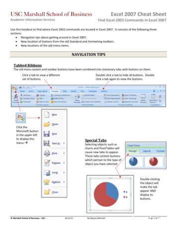
Excel 2007 Cheat Sheet Find Excel 2003 Commands in Excel 2007 Use this handout to find where Excel 2003 commands are located in Excel 2007. It consists of the following three sections: Navigation tips about getting around in Excel 2007. New location of buttons from the old Standard and
Microsoft Excel 2019 Formulas and Functions. Published with the authorization of Microsoft Corporation by: Pearson Education, Inc. . Formula limits in Excel 2019 . 4. Entering and editing formulas . 4. Using arithmetic formulas .
Excel 2013 Formulas and Functions Contents at a Glance Introduction Part I Mastering Excel Ranges and Formulas 1 Getting the Most Out of Ranges . 4 Creating Advanced Formulas


